Classes and Object Oriented Programming¶

In an earlier section we discussed classes as a way of representing an abstract object, such as a polynomial. The resulting code

[1]:

class Polynomial(object):
    """Representing a polynomial."""
    explanation = "I am a polynomial"

    def __init__(self, roots, leading_term):
        self.roots = roots
        self.leading_term = leading_term
        self.order = len(roots)

    def display(self):
        string = str(self.leading_term)
        for root in self.roots:
            if root == 0:
                string = string + "x"
            elif root > 0:
                string = string + "(x - {})".format(root)
            else:
                string = string + "(x + {})".format(-root)
        return string

    def multiply(self, other):
        roots = self.roots + other.roots
        leading_term = self.leading_term * other.leading_term
        return Polynomial(roots, leading_term)

    def explain_to(self, caller):
        print("Hello, {}. {}.".format(caller,self.explanation))
        print("My roots are {}.".format(self.roots))

allowed polynomials to be created, displayed, and multiplied together. However, the language is a little cumbersome. We can take advantage of a number of useful features of Python, many of which carry over to other programming languages, to make it easier to use the results.

Remember that the __init__ function is called when a variable is created. There are a number of special class functions, each of which has two underscores before and after the name. This is another Python convention that is effectively a rule: functions surrounded by two underscores have special effects, and will be called by other Python functions internally. So now we can create a variable that represents a specific polynomial by storing its roots and the leading term:

[2]:

p_roots = (1, 2, -3)
p_leading_term = 2
p = Polynomial(p_roots, p_leading_term)
p.explain_to("Alice")
q = Polynomial((1,1,0,-2), -1)
q.explain_to("Bob")

Hello, Alice. I am a polynomial.
My roots are (1, 2, -3).
Hello, Bob. I am a polynomial.
My roots are (1, 1, 0, -2).

Another special function that is very useful is __repr__. This gives a representation of the class. In essence, if you ask Python to print a variable, it will print the string returned by the __repr__ function. This was the role played by our display method, so we can just change the name of the function, making the Polynomial class easier to use. We can use this to create a simple string representation of the polynomial:

[3]:

class Polynomial(object):
    """Representing a polynomial."""
    explanation = "I am a polynomial"

    def __init__(self, roots, leading_term):
        self.roots = roots
        self.leading_term = leading_term
        self.order = len(roots)

    def __repr__(self):
        string = str(self.leading_term)
        for root in self.roots:
            if root == 0:
                string = string + "x"
            elif root > 0:
                string = string + "(x - {})".format(root)
            else:
                string = string + "(x + {})".format(-root)
        return string

    def explain_to(self, caller):
        print("Hello, {}. {}.".format(caller,self.explanation))
        print("My roots are {}.".format(self.roots))

[4]:

p = Polynomial(p_roots, p_leading_term)
print(p)
q = Polynomial((1,1,0,-2), -1)
print(q)

2(x - 1)(x - 2)(x + 3)
-1(x - 1)(x - 1)x(x + 2)

The final special function we’ll look at (although there are many more, many of which may be useful) is __mul__. This allows Python to multiply two variables together. We did this before using the multiply method, but by using the __mul__ method we can multiply together two polynomials using the standard * operator. With this we can take the product of two polynomials:

[5]:

class Polynomial(object):
    """Representing a polynomial."""
    explanation = "I am a polynomial"

    def __init__(self, roots, leading_term):
        self.roots = roots
        self.leading_term = leading_term
        self.order = len(roots)

    def __repr__(self):
        string = str(self.leading_term)
        for root in self.roots:
            if root == 0:
                string = string + "x"
            elif root > 0:
                string = string + "(x - {})".format(root)
            else:
                string = string + "(x + {})".format(-root)
        return string

    def __mul__(self, other):
        roots = self.roots + other.roots
        leading_term = self.leading_term * other.leading_term
        return Polynomial(roots, leading_term)

    def explain_to(self, caller):
        print("Hello, {}. {}.".format(caller,self.explanation))
        print("My roots are {}.".format(self.roots))

[6]:

p = Polynomial(p_roots, p_leading_term)
q = Polynomial((1,1,0,-2), -1)
r = p*q
print(r)

-2(x - 1)(x - 2)(x + 3)(x - 1)(x - 1)x(x + 2)

We now have a simple class that can represent polynomials and multiply them together, whilst printing out a simple string form representing itself. This can obviously be extended to be much more useful.

Inheritance¶

As we can see above, building a complete class from scratch can be lengthy and tedious. If there is another class that does much of what we want, we can build on top of that. This is the idea behind inheritance.

In the case of the Polynomial we declared that it started from the object class in the first line defining the class: class Polynomial(object). But we can build on any class, by replacing object with something else. Here we will build on the Polynomial class that we’ve started with.

A monomial is a polynomial whose leading term is simply 1. A monomial is a polynomial, and could be represented as such. However, we could build a class that knows that the leading term is always 1: there may be cases where we can take advantage of this additional simplicity.

We build a new monomial class as follows:

[7]:

class Monomial(Polynomial):
    """Representing a monomial, which is a polynomial with leading term 1."""

    def __init__(self, roots):
        self.roots = roots
        self.leading_term = 1
        self.order = len(roots)

Variables of the Monomial class are also variables of the Polynomial class, so can use all the methods and functions from the Polynomial class automatically:

[8]:

m = Monomial((-1, 4, 9))
m.explain_to("Caroline")
print(m)

Hello, Caroline. I am a polynomial.
My roots are (-1, 4, 9).
1(x + 1)(x - 4)(x - 9)

We note that these functions, methods and variables may not be exactly right, as they are given for the general Polynomial class, not by the specific Monomial class. If we redefine these functions and variables inside the Monomial class, they will override those defined in the Polynomial class. We do not have to override all the functions and variables, just the parts we want to change:

[9]:

class Monomial(Polynomial):
    """Representing a monomial, which is a polynomial with leading term 1."""
    explanation = "I am a monomial"

    def __init__(self, roots):
        self.roots = roots
        self.leading_term = 1
        self.order = len(roots)

    def __repr__(self):
        string = ""
        for root in self.roots:
            if root == 0:
                string = string + "x"
            elif root > 0:
                string = string + "(x - {})".format(root)
            else:
                string = string + "(x + {})".format(-root)
        return string

[10]:

m = Monomial((-1, 4, 9))
m.explain_to("Caroline")
print(m)

Hello, Caroline. I am a monomial.
My roots are (-1, 4, 9).
(x + 1)(x - 4)(x - 9)

This has had no effect on the original Polynomial class and variables, which can be used as before:

[11]:

s = Polynomial((2, 3), 4)
s.explain_to("David")
print(s)

Hello, David. I am a polynomial.
My roots are (2, 3).
4(x - 2)(x - 3)

And, as Monomial variables are Polynomials, we can multiply them together to get a Polynomial:

[12]:

t = m*s
t.explain_to("Erik")
print(t)

Hello, Erik. I am a polynomial.
My roots are (-1, 4, 9, 2, 3).
4(x + 1)(x - 4)(x - 9)(x - 2)(x - 3)

In fact, we can be a bit smarter than this. Note that the __init__ function of the Monomial class is identical to that of the Polynomial class, just with the leading_term set explicitly to 1. Rather than duplicating the code and modifying a single value, we can call the __init__ function of the Polynomial class directly. This is because the Monomial class is built on the Polynomial class, so knows about it. We regenerate the class, but only change the __init__ function:

[13]:

class Monomial(Polynomial):
    """Representing a monomial, which is a polynomial with leading term 1."""
    explanation = "I am a monomial"

    def __init__(self, roots):
        Polynomial.__init__(self, roots, 1)

    def __repr__(self):
        string = ""
        for root in self.roots:
            if root == 0:
                string = string + "x"
            elif root > 0:
                string = string + "(x - {})".format(root)
            else:
                string = string + "(x + {})".format(-root)
        return string

[14]:

v = Monomial((2, -3))
v.explain_to("Fred")
print(v)

Hello, Fred. I am a monomial.
My roots are (2, -3).
(x - 2)(x + 3)

We are now being very explicit in saying that a Monomial really is a Polynomial with leading_term being 1. Note, that in this case we are calling the __init__ function directly, so have to explicitly include the self argument.

By building on top of classes in this fashion, we can build classes that transparently represent the objects that we are interested in.

Most modern programming languages include some object oriented features. Many (including Python) will have more complex features than are introduced above. However, the key points where

a single variable representing an object can be defined,
methods that are specific to those objects can be defined,
new classes of object that inherit from and extend other classes can be defined,

are the essential steps that are common across nearly all.

Exercise: Equivalence classes¶

This exercise repeats that from the earlier chapter on classes, but explicitly includes new class methods to make equivalence classes easier to work with.

An equivalence class is a relation that groups objects in a set into related subsets. For example, if we think of the integers modulo $7$ , then $1$ is in the same equivalence class as $8$ (and $15$ , and $22$ , and so on), and $3$ is in the same equivalence class as $10$ . We use the tilde $3 \sim 10$ to denote two objects within the same equivalence class.

Here, we are going to define the positive integers programmatically from equivalent sequences.

Exercise 1¶

Define a Python class Eqint. This should be

Initialized by a sequence;
Store the sequence;
Define its representation (via the __repr__ function) to be the integer length of the sequence;
Redefine equality (via the __eq__ function) so that two Eqints are equal if their sequences have the same length.

Exercise 2¶

Define a zero object from the empty list, and three one objects, from a single object list, tuple, and string. For example

one_list = Eqint([1])
one_tuple = Eqint((1,))
one_string = Eqint('1')

Check that none of the one objects equal the zero object, but all equal the other one objects. Print each object to check that the representation gives the integer length.

Exercise 3¶

Redefine the class by including an __add__ method that combines the two sequences. That is, if a and b are Eqints then a+b should return an Eqint defined from combining a and bs sequences.

Note¶

Adding two different types of sequences (eg, a list to a tuple) does not work, so it is better to either iterate over the sequences, or to convert to a uniform type before adding.

Exercise 4¶

Check your addition function by adding together all your previous Eqint objects (which will need re-defining, as the class has been redefined). Print the resulting object to check you get 3, and also print its internal sequence.

Exercise 5¶

We will sketch a construction of the positive integers from nothing.

Define an empty list positive_integers.
Define an Eqint called zero from the empty list. Append it to positive_integers.
Define an Eqint called next_integer from the Eqint defined by a copy of positive_integers (ie, use Eqint(list(positive_integers)). Append it to positive_integers.
Repeat step 3 as often as needed.

Use this procedure to define the Eqint equivalent to $10$ . Print it, and its internal sequence, to check.

Exercise: Rational numbers¶

Instead of working with floating point numbers, which are not “exact”, we could work with the rational numbers $\mathbb{Q}$ . A rational number $q \in \mathbb{Q}$ is defined by the numerator $n$ and denominator $d$ as $q = \frac{n}{d}$ , where $n$ and $d$ are coprime (ie, have no common divisor other than $1$ ).

Exercise 1¶

Find a Python function that finds the greatest common divisor (gcd) of two numbers. Use this to write a function normal_form that takes a numerator and divisor and returns the coprime $n$ and $d$ . Test this function on $q = \frac{3}{2}$ , $q = \frac{15}{3}$ , and $q = \frac{20}{42}$ .

Exercise 2¶

Define a class Rational that uses the normal_form function to store the rational number in the appropriate form. Define a __repr__ function that prints a string that looks like $\frac{n}{d}$ (hint: use len(str(number)) to find the number of digits of an integer, and use \n to start a new line). Test it on the cases above.

Exercise 3¶

Overload the __add__ function so that you can add two rational numbers. Test it on $\frac{1}{2} + \frac{1}{3} + \frac{1}{6} = 1$ .

Exercise 4¶

Overload the __mul__ function so that you can multiply two rational numbers. Test it on $\frac{1}{3} \times \frac{15}{2} \times \frac{2}{5} = 1$ .

Exercise 5¶

Overload the `__rmul__ <https://docs.python.org/2/reference/datamodel.html?highlight=rmul#object.__rmul__>`__ function so that you can multiply a rational by an integer. Check that $\frac{1}{2} \times 2 = 1$ and $\frac{1}{2} + (-1) \times \frac{1}{2} = 0$ . Also overload the __sub__ function (using previous functions!) so that you can subtract rational numbers and check that $\frac{1}{2} - \frac{1}{2} = 0$ .

Exercise 6¶

Overload the __float__ function so that float(q) returns the floating point approximation to the rational number q. Test this on $\frac{1}{2}, \frac{1}{3}$ , and $\frac{1}{11}$ .

Exercise 7¶

Overload the __lt__ function to compare two rational numbers. Create a list of rational numbers where the denominator is $n = 2, \dots, 11$ and the numerator is the floored integer $n/2$ , ie n//2. Use the sorted function on that list (which relies on the __lt__ function).

Exercise 8¶

The Wallis formula for π is

$\pi = 2 \prod_{n=1}^{\infty} \frac{ (2 n)^2 }{(2 n - 1) (2 n + 1)}.$

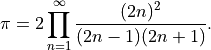
We can define a partial product $\pi_N$ as

$\pi_N = 2 \prod_{n=1}^{N} \frac{ (2 n)^2 }{(2 n - 1) (2 n + 1)},$

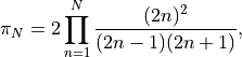
each of which are rational numbers.

Construct a list of the first 20 rational number approximations to $\pi$ and print them out. Print the sorted list to show that the approximations are always increasing. Then convert them to floating point numbers, construct a numpy array, and subtract this array from $\pi$ to see how accurate they are.

Classes and Object Oriented Programming¶

Inheritance¶

Exercise: Equivalence classes¶

Exercise 1¶

Exercise 2¶

Exercise 3¶

Note¶

Exercise 4¶

Exercise 5¶

Exercise: Rational numbers¶

Exercise 1¶

Exercise 2¶

Exercise 3¶

Exercise 4¶

Exercise 5¶

Exercise 6¶

Exercise 7¶

Exercise 8¶

Maths with Python

Navigation

Related Topics