Loops

while loops

The program we wrote at the end of the last part performs a series of repetitive operations, but did it by copying and pasting the call to our function and editing the input. As noted above, this is a likely source of errors. Instead we want to write a formula, algorithm or abstraction of our repeated operation, and reproduce that in code.

First we reproduce that function:

from math import pi

def degrees_to_radians(theta_d):
    """
    Convert an angle from degrees to radians.

    Parameters
    ----------

    theta_d : float
        The angle in degrees.

    Returns
    -------

    theta_r : float
        The angle in radians.
    """
    theta_r = pi / 180.0 * theta_d
    return theta_r

We showed above how to use this code to print the angles for . We did this by calling the degrees_to_radians function on the angles degrees for . So this is the formula we want to reproduce in code. To do that we write a loop.

Here is a standard way to do it:

theta_d = 0.0
while theta_d <= 90.0:
    print(degrees_to_radians(theta_d))
    theta_d = theta_d + 15.0

0.0
0.2617993877991494
0.5235987755982988
0.7853981633974483
1.0471975511965976
1.3089969389957472
1.5707963267948966

Let’s examine this line by line. The first line defines the angle in degrees, theta_d. We start from .

The next line defines the loop. This has similarities to our definition of a function. We use the keyword while to say that what follows is going to be a loop. We then define a logical condition that will be either True or False. Whilst the condition is True, the statements in the loop will be executed. The colon : at the end of the line ends the logical condition and says that what follows will be the statements inside the loop. As with the function, the code block with the statements inside the loop is indented by four spaces or one tab.

The code block contains two lines, both of which will be executed. The first prints the converted angle to the screen. The second increases the angle in degrees by 15. At the end of the code block, Python will check the logical condition theta_d <= 90.0 again. If it is True the statements inside the loop are executed again. If it is False, the code moves on to the next line after the loop.

There is another way to write a loop that we can use:

for loops

steps = 1, 2, 3, 4, 5, 6
for n in steps:
    print(degrees_to_radians(15*n))

0.2617993877991494
0.5235987755982988
0.7853981633974483
1.0471975511965976
1.3089969389957472
1.5707963267948966

Let’s examine this code line by line. It first defines a set of numbers, steps, which contains the integers from 1 to 6 (we will make this more precise later when we discuss lists and tuples). We then define the loop using the for command. This looks at the set of numbers steps and picks an entry out one at a time, setting the variable n to be the value of that member of the set. So, the first time through the loop n=1. The next, n=2. Once it has iterated through all members of the set steps, it stops.

The colon : at the end of the line defines the code block that each iteration of the loop should perform. Exactly as when we defined a function, the code block is indented by four spaces or one tab. In each iteration through the loop, the commands indented by this amount will be run. In this case, only one line (the print... line) will be run. On each iteration the value of n changes, leading to the different angle.

Writing out a long list of integers is a bad idea. A better approach is the use the range function. This compresses the code to:

for n in range(1,7):
    print(degrees_to_radians(15*n))

0.2617993877991494
0.5235987755982988
0.7853981633974483
1.0471975511965976
1.3089969389957472
1.5707963267948966

The range function takes the input arguments <start> and <end>, and the optional input argument <step>, to produce the integers from the start up to, but not including, the end. If the <start> is not given it defaults to 0, and if the <step> is not given it defaults to 1.

(Strictly, range does not return the full list in one go. It generates the results one at a time. This is much faster and more efficient. In the for loop this is all you need. To actually view what range generates all together, convert it to a list, as list(range(...))).

Check this against examples such as:

print(list(range(4)))
print(list(range(-1,3)))
print(list(range(1,10,2)))

[0, 1, 2, 3]
[-1, 0, 1, 2]
[1, 3, 5, 7, 9]

In some programming languages this is where the discussion of a for loop would end: the “loop counter” must be an integer. In Python, a loop is just iterating over a set of values, and these can be much more general. An alternative way (using floats) to do the same loop would be

angles = 15.0, 30.0, 45.0, 60.0, 75.0, 90.0
for angle in angles:
    print(degrees_to_radians(angle))

0.2617993877991494
0.5235987755982988
0.7853981633974483
1.0471975511965976
1.3089969389957472
1.5707963267948966

But we can get much more general than that. The different things in the set don’t have to have the same type:

things = 1, 2.3, True, degrees_to_radians
for thing in things:
    print(thing)

1
2.3
True
<function degrees_to_radians at 0x104b4fbf8>

This can be used to write very efficient code, but is a feature that isn’t always available in other programming languages.

When should we use for loops and when while loops? In most cases either will work. Different algorithms have different conventions, so where possible follow the convention. The advantage of the for loop is that it is clearer how much work will be done by the loop (as, in principle, we know how many times the loop block will be executed). However, sometimes you need to perform a repetitive operation but don’t know in advance how often you’ll need to do it. For example, to the nearest degree, what is the largest angle that when converted to radians is less than 4? (For the picky, we’re restricting so that ).

Rather than doing the sensible thing and doing the analytic calculation, we can do the following:

1. Set .
2. Calculate the angle in radians .
3. If :
   • Increase by ;
   • Repeat from step 2.

We can reproduce this algorithm using a while loop:

theta_d = 0.0

while degrees_to_radians(theta_d) < 4.0:
    theta_d = theta_d + 1.0

This could be done in a for loop, but not so straightforwardly.

To summarize:

The structure of the while loop is similar to the for loop. The loop is defined by a keyword (while or for) and the end of the line defining the loop condition is given by a colon. With each iteration of the loop the indented code is executed. The difference is in how the code decides when to stop looping, and what changes with each iteration.

In the for loop the code iterates over the objects in a set, and some variable is modified with each iteration based on the new object. Once all objects in the set have been iterated over, the loop stops.

In a while loop some condition is checked; while it is true the loop continues, and as soon as it is false the loop stops. Here we are checking if , given by degrees_to_radians(theta_d), is still less than 4. However, nothing in the definition of the loop actually changes: it is the statement within the loop that actually changes the angle .

We quickly check that the answer given makes sense:

print(theta_d - 1.0)
print(theta_d)
print(degrees_to_radians(theta_d-1.0) / 4.0)
print(degrees_to_radians(theta_d) / 4.0)

229.0
230.0
0.9992009967667537
1.0035643198967394

We see that the answer is .

Logical statements

We noted above that whether or not a while loop executes depends on the truth (or not) of a particular statement. In programming these logical statements take Boolean values (either true or false). In Python, the values of a Boolean statement are either True or False, which are the keywords used to refer to them. Multiple statements can be chained together using the logical operators and, or, not. For example:

print(True)
print(6 < 7 and 10 > 9)
print(1 < 2 or 1 < 0)
print(not (6 < 7) and 10 > 9)
print(6 < 7 < 8)

True
True
True
False
True

The last example is particularly important, as this chained example (6 < 7 < 8) is equivalent to (6 < 7) and (7 < 8). This checks both inequalities - checking that when , by checking that both and is true when , which is true (and mathematically what you would expect). However, many programming languages would not interpret it this way, but would instead interpret it as (6 < 7) < 8, which is equivalent to True < 8, which is nonsense. Chaining operations in this way is useful in Python, but don’t expect it to always work in other languages.

Containers and Sequences

When talking about loops we informally introduced the collection of objects 1, 2, 3, 4, 5, 6, and assigned it to a single variable steps. This is one of many types of container: a single object that contains other objects. If the objects in the container have an order then the container is often called a sequence: an object that contains an ordered sequence of other objects. These sorts of objects are everywhere in mathematics: sets, groups, vectors, matrices, equivalence classes, categories, … Programming languages also implement a large number of them. Python has four essential containers, the most important of which for our purposes are lists, tuples, and dictionaries.

Lists

A list is an ordered collection of objects. For example:

list1 = [1, 2, 3, 4, 5, 6]
list2 = [15.0, 30.0, 45.0, 60.0, 75.0, 90.0]
list3 = [1, 2.3, True, degrees_to_radians]
list4 = ["hello", list1, False]
list5 = []

Lists are defined by square brackets, []. Objects in the list are separated by commas. A list can be empty (list5 above). A list can contain other lists (list4 above). The objects in the list don’t have to have the same type (list3 and list4 above).

We can access a member of a list by giving its name, square brackets, and the index of the member (starting from 0!):

list1[0]

1

list2[3]

60.0

Note

There is a big divide between programming languages that index containers (or vectors, or lists) starting from 0 and those that index starting from 1. There is no consensus on which is better, so as you move between languages, get used to checking which is used.

Entries in a list can be modified:

list4[1] = "goodbye"
list4

['hello', 'goodbye', False]

Additional entries can be appended onto the end of a list:

list4.append('end')
list4

['hello', 'goodbye', False, 'end']

Entries can be removed (popped) from the end of a list:

entry = list4.pop()
print(entry)
list4

end

['hello', 'goodbye', False]

The length of a list can be found:

len(list4)

3

Lists are probably the most used container, but there’s a closely related container that we’ve already used: the tuple.

Tuples

Tuples are ordered collections of objects that, once created, cannot be modified. For example:

tuple1 = 1, 2, 3, 4, 5, 6
tuple2 = (15.0, 30.0, 45.0, 60.0, 75.0, 90.0)
tuple3 = (1, 2.3, True, degrees_to_radians)
tuple4 = ("hello", list1, False)
tuple5 = ()
tuple6 = (5,)

Tuples are defined by the commas separating the entries. The round brackets () surrounding the entries are conventional, useful for clarity, and for grouping. If you want to create an empty tuple (tuple5) the round brackets are necessary. A tuple containing a single entry (tuple6) must have a trailing comma.

Tuples can be accessed in the same ways as lists, and their length found with len in the same way. But they cannot be modified, so we cannot add additional entries, or remove them, or alter any:

tuple1[0]

1

tuple4[1] = "goodbye"

---------------------------------------------------------------------------
TypeError                                 Traceback (most recent call last)
<ipython-input-20-954f9f41259d> in <module>()
----> 1 tuple4[1] = "goodbye"

TypeError: 'tuple' object does not support item assignment

However, if a member of a tuple can itself be modified (for example, it’s a list, as tuple4[1] is), then that entry can be modified:

print(tuple4[1])
tuple4[1][1] = 33
print(tuple4[1])

[1, 2, 3, 4, 5, 6]
[1, 33, 3, 4, 5, 6]

Tuples appear a lot when using functions, either when passing in parameters, or when returning results. They can often be treated like lists, and there are functions that convert lists to tuples and vice versa:

converted_list1 = list(tuple1)
converted_tuple1 = tuple(list1)

Slicing

Accessing and manipulating multiple entries of a list at once is an efficient and effective way of coding: it shows up a lot in, for example, linear algebra. This is where slicing comes in.

We have seen that we can access a single element of a list using square brackets and an index. We can use similar notation to access multiple elements:

list1 = [1, 2, 3, 4, 5, 6]
print(list1[0])
print(list1[1:3])
print(list1[2:])
print(list1[:4])

1
[2, 3]
[3, 4, 5, 6]
[1, 2, 3, 4]

The slicing notation [<start>:<end>] returns all entries from the <start> to the entry before the <end>. So:

• list1[1:3] returns all entries from the second (index 1) to the third (the entry before index 3).
• if <end> is not given all entries up to the end are returned, so list1[2:] returns all entries from the third (index 2) to the end.
• if <start> is not given all entries from the start are returned, so list1[:4] returns all entries from the start until the fourth (the entry before index 4).

There are a number of other ways that slicing can be used. First, we can specify the step:

print(list1[0:6:2])
print(list1[1::3])
print(list1[4:1:-1])

[1, 3, 5]
[2, 5]
[5, 4, 3]

By using a negative step we can reverse the order (as shown in the final example), but then we need to be careful with the <start> and <end>.

This <start>:<end>:<step> notation varies between programming languages: some use <start>:<step>:<end>.

Second, we can give an index that counts from the end, where the final entry is -1:

print(list1[-1])
print(list1[-2])
print(list1[2:-2])
print(list1[-4:-2])

6
5
[3, 4]
[3, 4]

Unpacking

Slicing is often seen as part of assignment. For example

list_slice = [0, 0, 0, 0, 0, 0, 0, 0]
list_slice[1:4] = list1[3:]
print(list_slice)

[0, 4, 5, 6, 0, 0, 0, 0]

This is related to a very useful Python feature: unpacking. Normally we have assigned a single variable to a single value (although that value might be a container such as a list). However, we can assign multiple values in one go:

a, b, c = list1[3:]
print(a)
print(b)
print(c)

4
5
6

This can be used to directly swap two variables, for example:

a, b = b, a
print(a)
print(b)

5
4

The number of entries on both sides must match.

Dictionaries

All the containers we have seen so far have had an order - lists and tuples are sequences, and we access the objects within them using list[0] or tuple[3], for example. A dictionary is our first unordered container. These are useful for collections of objects with meaningful names, but where the order of the objects has no importance.

Dictionaries are defined using curly braces. The “name” of each entry is given first (usually called its key), followed by a :, and then after the colon comes its value. Multiple entries are separated by commas. For example:

from math import sin, cos, exp, log

functions = {"sine" : sin,
             "cosine" : cos,
             "exponential" : exp,
             "logarithm" : log}

print(functions)

{'sine': <built-in function sin>, 'exponential': <built-in function exp>, 'logarithm': <built-in function log>, 'cosine': <built-in function cos>}

Note that the order it prints out need not match the order we entered the values in. In fact, the order could change if we used a different machine, or entered the values again. This emphasizes the unordered nature of dictionaries.

To access an individual value, we use its key:

print(functions["exponential"])

<built-in function exp>

To find all the keys or values we can use dictionary methods:

print(functions.keys())
print(functions.values())

dict_keys(['sine', 'exponential', 'logarithm', 'cosine'])
dict_values([<built-in function sin>, <built-in function exp>, <built-in function log>, <built-in function cos>])

Depending on the version of Python you are using, this might either give a list or an iterator.

When iterating over a dictionary (for k in dict:) the key is returned, as if we had said for key in dict.keys():. This is most useful in a loop, such as the following. Think carefully about this code, and make sure you understand what is happening!

for name in functions:
    print("The result of {}(1) is {}.".format(name, functions[name](1.0)))

The result of sine(1) is 0.8414709848078965.
The result of exponential(1) is 2.718281828459045.
The result of logarithm(1) is 0.0.
The result of cosine(1) is 0.5403023058681398.

To explain: The first line says that we are going to iterate over each entry in the dictionary by assigning the value of the key (which is the name of the function in functions) to the variable name. The next line extracts the function associated with that name using functions[name] and applies that function to the value 1 using functions[name](1.0). The full line prints out the result in a human readable form.

But Python has other ways of iterating over dictionaries that can make life even easier, such as the items function:

for name, function in functions.items():
    print("The result of {}(1) is {}.".format(name, function(1.0)))

The result of sine(1) is 0.8414709848078965.
The result of exponential(1) is 2.718281828459045.
The result of logarithm(1) is 0.0.
The result of cosine(1) is 0.5403023058681398.

So this does exactly the same thing as the previous loop, and most of the code is the same. However, rather than accessing the dictionary each time (using functions[name]), the value in the dictionary has been returned at the start. What is happening is that the items function is returning both the key and the value as a tuple on each iteration through the loop. The name, function notation then uses unpacking to appropriately set the variables. This form is “more pythonic” (ie, is shorter, clearer to many people, and faster).

Above we have always set the key to be a string. This is not necessary - it can be an integer, or a float, or any constant object. We have also set the values to have the same type. As with lists this is not necessary.

Dictionaries are very useful for adding simple structure to your code, and allow you to pass around complex sets of parameters easily.

Control flow

Not every algorithm can be expressed as a single mathematical formula in the manner used so far. Alternatively, it may make the algorithm appear considerably simpler if it isn’t expressed in one complex formula but in multiple simpler forms. This is where the computer has to be able to make choices, to control when and if a particular formula is used.

As a simple example, if we used our degrees_to_radians calculation as previously given, then if the angle is outside the standard interval then the converted angle in radians will be outside the interval.

Suppose we want to “normalize” all our angles to lie within the interval. We could use modular arithmetic using the % operator:

theta_d = 5134.6
theta_d_normalized = theta_d % 360.0
print(theta_d_normalized)

94.60000000000036

But it might be that the input is just wrong: there’s a typo, and the caller should be warned, and maybe the input completely rejected. We can write a different function to check that.

from math import pi

def check_angle_normalized(theta_d):
    """
    Check that an angle lies within [0, 360] degrees.

    Parameters
    ----------

    theta_d : float
        The angle in degrees.

    Returns
    -------

    normalized : Boolean
        Whether the angle lies within the range
    """

    normalized = True
    if theta_d > 360.0:
        normalized = False
        print("Input angle greater than 360 degrees. Did you mean this?")
    if theta_d < 0.0:
        normalized = False
        print("Input angle less than 0 degrees. Did you mean this?")
    return normalized

theta_d = 5134.6
print(check_angle_normalized(theta_d))
theta_d = -52.3
print(check_angle_normalized(theta_d))

Input angle greater than 360 degrees. Did you mean this?
False
Input angle less than 0 degrees. Did you mean this?
False

The control flow here uses the if statement. As with loops such as the for and while loops we have a condition which is checked which, if satisfied, leads to the indented code block after the colon being executed. The logical statements theta_d > 360.0 and theta_d < 0.0 are evaluated and return either True or False (which is how Python represents boolean values). If True, then the statement is executed.

We could use only a single logical statement to check if lies in an acceptable range by using logical relations. For example, we could replace the two if statements by the single statement

if (theta_d > 360.0) or (theta_d < 0.0):
    normalized = False
    print("Input angle outside [0, 360] degrees. Did you mean this?")

The logical statement (theta_d > 360.0) or (theta_d < 0.0) is either True or False as above. In addition to the logical or statement, Python also has the logical and and logical not statements, from which more complex statements can be generated.

Often we want to do one thing if a condition is true, and another if the condition is false. A full example of this would be to rewrite the whole function as:

from math import pi

def check_angle_normalized(theta_d):
    """
    Check that an angle lies within [0, 360] degrees.

    Parameters
    ----------

    theta_d : float
        The angle in degrees.

    Returns
    -------

    normalized : Boolean
        Whether the angle lies within the range
    """

    normalized = True
    if theta_d > 360.0:
        normalized = False
        print("Input angle greater than 360 degrees. Did you mean this?")
    elif theta_d < 0.0:
        normalized = False
        print("Input angle less than 0 degrees. Did you mean this?")
    else:
        print("Input angle in range [0, 360] degrees. Good.")
    return normalized

The elif statement allows another condition to be checked - it is how Python represents “else if”, or “all previous checks have been false; let’s check this statement as well”. Multiple elif blocks can be included to check more conditions. The else statement contains no logical check: this code block will always be executed if all previous statements were false.

For example:

theta_d = 543.2
print(check_angle_normalized(theta_d))
theta_d = -123.4
print(check_angle_normalized(theta_d))
theta_d = 89.12
print(check_angle_normalized(theta_d))

Input angle greater than 360 degrees. Did you mean this?
False
Input angle less than 0 degrees. Did you mean this?
False
Input angle in range [0, 360] degrees. Good.
True

We can nest statements as deep as we like, nesting loops and control flow statements as we go. We have to ensure that the indentation level is consistent. Here is a silly example.

angles = [-123.4, 543.2, 89.12, 0.67, 5143.6, 30.0, 270.0]

# We run through all the angles, but only print those that are
# - in the range [0, 360], and
# - if sin^2(angle) < 0.5

from math import sin

for angle in angles:
    print("Input angle in degrees:", angle)
    if (check_angle_normalized(angle)):
        angle_r = degrees_to_radians(angle)
        if (sin(angle_r)**2 < 0.5):
            print("Valid angle in radians:", angle_r)

Input angle in degrees: -123.4
Input angle less than 0 degrees. Did you mean this?
Input angle in degrees: 543.2
Input angle greater than 360 degrees. Did you mean this?
Input angle in degrees: 89.12
Input angle in range [0, 360] degrees. Good.
Input angle in degrees: 0.67
Input angle in range [0, 360] degrees. Good.
Valid angle in radians: 0.011693705988362009
Input angle in degrees: 5143.6
Input angle greater than 360 degrees. Did you mean this?
Input angle in degrees: 30.0
Input angle in range [0, 360] degrees. Good.
Valid angle in radians: 0.5235987755982988
Input angle in degrees: 270.0
Input angle in range [0, 360] degrees. Good.

Debugging

Earlier we saw how to read error messages to debug single statements. When we start including loops and functions it may be more complex and the information from the error message alone, whilst useful, may not be enough.

In these more complex cases the reason for the error depends on the calculations inside the code, and the steps through the code need inspecting in detail. This is where a debugger is useful. It allows you to run the code, pause at specific points or conditions, step through it as it runs line-by-line, and inspect all the values as you go. There are a number of Python debuggers - pdb and ipdb being the most basic. However, spyder has a debugger built in, and learning to use it will make your life considerably easier.

Breakpoints

The main use of the debugger is to inspect the internal state of a code whilst it is running. To do that we have to stop the execution of the code somewhere. This is typically done using breakpoints.

Copy the following function into a file named breakpoints.py:

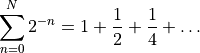
def test_sequence(N):
    """
    Compute the infinite sum of 2^{-n} starting from n = 0, truncating
    at n = N, returning the value of 2^{-n} and the truncated sum.

    Parameters
    ----------

    N : int
        Positive integer, giving the number of terms in the sum

    Returns
    -------

    limit : float
        The value of 2^{-N}
    partial_sum : float
        The value of the truncated sum

    Notes
    -----

    The limiting value should be zero, and the value of the sum should
    converge to 2.
    """

    # Start sum from zero, so give zeroth term
    limit = 1.0
    partial_sum = 1.0

    # At each step, increment sum and change summand
    for n in range(1, N+1):
        partial_sum = partial_sum + limit
        limit = limit / 2.0

    return limit, partial_sum

if __name__ == '__main__':
    print(test_sequence(50))

This computes the value and the partial sum . The limit as of the value should be zero, and of the sum should be two.

The final two lines ensures that, if the file is run as a python script, the function will be called (with N=50). The if statement is a standard Python convention: if you have code that you want executed only if the file is run as a script, and not if the file is imported as a module.

If we run the function we find it does not work as expected:

import breakpoints
print(breakpoints.test_sequence(10))
print(breakpoints.test_sequence(100))
print(breakpoints.test_sequence(1000))

(0.0009765625, 2.998046875)
(7.888609052210118e-31, 3.0)
(9.332636185032189e-302, 3.0)

The value is tending to the right limit; the sum is not. The test (that we should have written formally) has failed. It may be obvious what the problem is, but we illustrate how to find it using the debugger.

First, we must know what to expect. The terms in the partial sum (which is where the problem lies) should be

We want to inspect what the partial sum actually does. This is performed in the code within the for loop, which starts on line 32 of the code.

1. Open the code in spyder.
2. Ensure that the working directory is set to the directory the file is in (shortcut: the top right corner of the editor part of the window contains a drop down “Options” menu: the second option “Set console working directory” will do what is needed.)
3. Set a breakpoint on line 32. To do this, double-click on the “32” on the left hand side of the editor screen. A small red circle will appear next to it. (To remove a breakpoint, double click the number again)
4. Start debugging by going to the “Debug” menu and clicking “Debug”. The console will indicate that
   1. The code has been started
   2. The code has paused at line 32.
5. In the top right of the spyder window, click on the “Variable explorer” tab. This shows the values of all the variables at this point. Note that line 32 has not yet been executed. The value of the partial sum, given by partial_sum, is currently 1 (as the N=0 term is set outside of the sum).
6. Work out which toolbar button “Runs” the current line. You should see
   1. The “active line” marker in the editor and console move forward to line 33;
   2. The value of the loop counter n appear in the Variable explorer, set to 1.
7. “Run” the current line again (which will now be line 33). We see that it adds the current value of limit, which is meant to represent , to the partial sum partial_sum. However, this value is 1, so partial_sum becomes 2. According to the sum written out above, this term should be . So this is a bug.

To fix this bug, the simplest thing to do is to ensure that limit has the value corresponding to the nth part of the sum before it is used, by swapping lines 33 and 34.

You should experiment with adding breakpoints and stepping through some of your own codes. In particular, you should note that “Run”ning the current line of code will skip over any function calls, including calls to functions you have yourself defined. If you want to follow the code as it executes functions, you need to use the “Step into” button instead.

Exercise: Prime numbers

Exercise 1

Write a function that tests if a number is prime. Test it by writing out all prime numbers less than 50.

Hint: if b divides a then a % b == 0 is True.

Exercise 2

500 years ago some believed that the number was prime for all primes . Use your function to find the first prime for which this is not true.

Exercise 3

The Mersenne primes are those that have the form , where is prime. Use your previous solutions to generate all the that give Mersenne primes.

Exercise 4

Write a function to compute all prime factors of an integer , including their multiplicities. Test it by printing the prime factors (without multiplicities) of and the multiplicities (without factors) of .

Note

One effective solution is to return a dictionary, where the keys are the factors and the values are the multiplicities.

Exercise 5

Write a function to generate all the integer divisors, including 1, but not including itself, of an integer . Test it on .

Note

You could use the prime factorization from the previous exercise, or you could do it directly.

Exercise 6

A perfect number is one where the divisors sum to . For example, 6 has divisors 1, 2, and 3, which sum to 6. Use your previous solution to find all perfect numbers (there are only four!).

Exercise 7

Using your previous functions, check that all perfect numbers can be written as , where is a Mersenne prime.

Exercise 8 (bonus)

Investigate the timeit function in Python or IPython. Use this to measure how long your function takes to check that, if on the Mersenne list then is a perfect number, using your functions. Stop increasing when the time takes too long!

Note

You could waste considerable time on this, and on optimizing the functions above to work efficiently. It is not worth it, other than to show how rapidly the computation time can grow!