Programs¶

Using the Python console to type in commands works fine, but has serious drawbacks. It doesn’t save the work for the future. It doesn’t allow the work to be re-used. It’s frustrating to edit when you make a mistake, or want to make a small change. Instead, we want to write a program.

A program is a text file containing Python commands. It can be written in any text editor. Something like the editor in spyder is ideal: it has additional features for helping you write code. However, any plain text editor will work. A program like Microsoft Word will not work, as it will try and save additional information with the file.

Let us use a simple pair of Python commands:

[1]:

import math
x = math.sin(1.2)

Go to the editor in spyder and enter those commands in a file:

import math
x = math.sin(1.2)

Save this file in a suitable location and with a suitable name, such as lab1_basic.py (the rules and conventions for filenames are similar to those for variable names laid out above: descriptive, lower case names without spaces). The file extension should be .py: spyder should add this automatically.

To run this program, either

press the green “play” button in the toolbar;
press the function key F5;
select “Run” from the “Run” menu.

In the console you should see a line like

runfile('/Users/ih3/PythonLabs/lab1_basic.py', wdir='/Users/ih3/PythonLabs')

appear, and nothing else. To check that the program has worked, check the value of x. In the console just type x:

[2]:

[2]:

0.9320390859672263

Also, in the top right of the spyder window, select the “Variable explorer” tab. It shows the variables that it currently knows, which should include x, its type (float) and its value.

If there are many variables known, you may worry that your earlier tests had already set the value for x and that the program did not actually do anything. To get back to a clean state, type %reset in the console to delete all variables - you will need to confirm that you want to do this. You can then re-run the program to test that it worked.

Using programs and modules¶

In previous sections we have imported and used standard Python libraries, packages or modules, such as math. This is one way of using a program, or code, that someone else has written. To do this for ourselves, we use exactly the same syntax.

Suppose we have the file lab1_basic.py exactly as above. Write a second file containing the lines

import lab1_basic
print(lab1_basic.x)

Save this file, in the same directory as lab1_basic.py, say as lab1_import.py. When we run this program, the console should show something like

runfile('/Users/ih3/PythonLabs/lab1_import.py', wdir='/Users/ih3/PythonLabs')
0.9320390859672263

This shows what the import statement is doing. All the library imports, definitions and operations in the imported program (lab1_basic) are performed. The results are then available to us, using the dot notation, via lab1_basic.<variable>, or lab1_basic.<function>.

To build up a program, we write Python commands into plain text files. When we want to use, or re-use, those definitions or results, we use import on the name of the file to recover their values.

Note¶

We saved both files - the original lab1_basic.py, and the program that imported lab1_basic.py, in the same directory. If they were in different directories then Python would not know where to find the file it was trying to import, and would give an error. The solution to this is to create a package, which is rather more work.

Functions¶

We have already seen and used some functions, such as the log and sin functions from the math package. However, in programming, a function is more general; it is any set of commands that acts on some input parameters and returns some output.

Functions are central to effective programming, as they stop you from having to repeat yourself and reduce the chances of making a mistake. Defining and using your own functions is the next step.

Let us write a function that converts angles from degrees to radians. The formula is

$\theta_r = \frac{\pi}{180} \theta_d,$

where $\theta_r$ is the angle in radians, and $\theta_d$ is the angle in degrees. If we wanted to do this for, eg, $\theta_d = 30^{\circ}$ , we could use the commands

[3]:

from math import pi
theta_d = 30.0
theta_r = pi / 180.0 * theta_d

[4]:

print(theta_r)

0.5235987755982988

This is effective for a single angle. If we want to repeat this for many angles, we could copy and paste the code. However, this is dangerous. We could make a mistake in editing the code. We could find a mistake in our original code, and then have to remember to modify every location where we copied it to. Instead we want to have a single piece of code that performs an action, and use that piece of code without modification whenever needed.

This is summarized in the “DRY” principle: do not repeat yourself. Instead, convert the code into a function and use the function.

We will define the function and show that it works, then discuss how:

[5]:

from math import pi

def degrees_to_radians(theta_d):
    """
    Convert an angle from degrees to radians.

    Parameters
    ----------

    theta_d : float
        The angle in degrees.

    Returns
    -------

    theta_r : float
        The angle in radians.
    """
    theta_r = pi / 180.0 * theta_d
    return theta_r

We check that it works by printing the result for multiple angles:

[6]:

print(degrees_to_radians(30.0))
print(degrees_to_radians(60.0))
print(degrees_to_radians(90.0))

0.5235987755982988
1.0471975511965976
1.5707963267948966

How does the function definition work?

First we need to use the def command:

def degrees_to_radians(theta_d):

This command effectively says “what follows is a function”. The first word after def will be the name of the function, which can be used to call it later. This follows similar rules and conventions to variables and files (no spaces, lower case, words separated by underscores, etc.).

After the function name, inside brackets, is the list of input parameters. If there are no input parameters the brackets still need to be there. If there is more than one parameter, they should be separated by commas.

After the bracket there is a colon :. The use of colons to denote special “blocks” of code happens frequently in Python code, and we will see it again later.

After the colon, all the code is indented by four spaces or one tab. Most helpful text editors, such as the spyder editor, will automatically indent the code after a function is defined. If not, use the tab key to ensure the indentation is correct. In Python, whitespace and indentation is essential: it defines where blocks of code (such as functions) start and end. In other languages special keywords or characters may be used, but in Python the indentation of the code statements is the key.

The statement on the next few lines is the function documentation, or docstring.

"""
Convert an angle from degrees to radians.

...
"""

This is in principle optional: it’s not needed to make the code run. However, documentation is extremely useful for the next user of the code. As the next user is likely to be you in a week (or a month), when you’ll have forgotten the details of what you did, documentation helps you first. In reality, you should always include documentation.

The docstring can be any string within quotes. Using “triple quotes” allows the string to go across multiple lines. The docstring can be rapidly printed using the help function:

[7]:

help(degrees_to_radians)

Help on function degrees_to_radians in module __main__:

degrees_to_radians(theta_d)
    Convert an angle from degrees to radians.

    Parameters
    ----------

    theta_d : float
        The angle in degrees.

    Returns
    -------

    theta_r : float
        The angle in radians.

This allows you to quickly use code correctly without having to look at the code. We can do the same with functions from packages, such as

[8]:

help(math.sin)

Help on built-in function sin in module math:

sin(...)
    sin(x)

    Return the sine of x (measured in radians).

You can put whatever you like in the docstring. The format used above in the degrees_to_radians function follows the numpydoc convention, but there are other conventions that work well. One reason for following this convention can be seen in spyder. Copy the function degrees_to_radians into the console, if you have not done so already. Then, in the top right part of the window, select the “Object inspector” tab. Ensure that the “Source” is “Console”. Type degrees_to_radians into the “Object” box. You should see the help above displayed, but nicely formatted.

You can put additional comments in your code - anything after a “#” character is a comment. The advantage of the docstring is how it can be easily displayed and built upon by other programs and bits of code, and the conventions that make them easier to write and understand.

Going back to the function itself. After the comment, the code to convert from degrees to radians starts. Compare it to the original code typed directly into the console. In the console we had

from math import pi
theta_d = 30.0
theta_r = pi / 180.0 * theta_d

In the function we have

theta_r = pi / 180.0 * theta_d
return theta_r

The line

from math import pi

is in the function file, but outside the definition of the function itself.

There are four differences.

The function code is indented by four spaces, or one tab.
The input parameter theta_d must be defined in the console, but not in the function. When the function is called the value of theta_d is given, but inside the function itself it is not: the function knows that the specific value of theta_d will be given as input.
The output of the function theta_r is explicitly returned, using the return statement.
The import statement is moved outside the function definition - this is the convention recommended by PEP8.

Aside from these points, the code is identical. A function, like a program, is a collection of Python statements exactly as you would type into a console. The first three differences above are the essential differences to keep in mind: the first is specific to Python (other programming languages have something similar), whilst the other differences are common to most programming languages.

Names used internally by the function are not visible externally. Also, the name used for the output of the function need not be used externally. To see an example of this, start with a clean slate by typing %reset into the console.

[9]:

%reset -f

Then copy and paste the function definition again:

[10]:

from math import pi

def degrees_to_radians(theta_d):
    """
    Convert an angle from degrees to radians.

    Parameters
    ----------

    theta_d : float
        The angle in degrees.

    Returns
    -------

    theta_r : float
        The angle in radians.
    """
    theta_r = pi / 180.0 * theta_d
    return theta_r

(Alternatively you can use the history in the console by pressing the up arrow until the definition of the function you previously entered appears. Then click at the end of the function and press Return). Now call the function as

[11]:

angle = degrees_to_radians(45.0)

[12]:

print(angle)

0.7853981633974483

But the variables used internally, theta_d and theta_r, are not known outside the function:

[13]:

theta_d

---------------------------------------------------------------------------
NameError                                 Traceback (most recent call last)
<ipython-input-13-a78047e2dfdf> in <module>()
----> 1 theta_d

NameError: name 'theta_d' is not defined

This is an example of scope: the existence of variables, and their values, is restricted inside functions (and files).

You may note that above, we had a value of theta_d outside the function (from when we were working in the console), and a value of theta_d inside the function (as the input parameter). These do not have to match. If a variable is assigned a value inside the function then Python will take this “local” value. If not, Python will look outside the function. Two examples will illustrate this:

[14]:

x1 = 1.1

def print_x1():
    print(x1)

print(x1)
print_x1()

1.1
1.1

[15]:

x2 = 1.2

def print_x2():
    x2 = 2.3
    print(x2)

print(x2)
print_x2()

1.2
2.3

In the first (x1) example, the variable x1 was not defined within the function, but it was used. When x1 is printed, Python has to look for the definition outside of the scope of the function, which it does successfully.

In the second (x2) example, the variable x2 is defined within the function. The value of x2 does not match the value of the variable with the same name defined outside the function, but that does not matter: within the function, its local value is used. When printed outside the function, the value of x2 uses the external definition, as the value defined inside the function is not known (it is “not in scope”).

Some care is needed with using scope in this way, as Python reads the whole function at the time it is defined when deciding scope. As an example:

[16]:

x3 = 1.3

def print_x3():
    print(x3)
    x3 = 2.4

print(x3)
print_x3()

1.3

---------------------------------------------------------------------------
UnboundLocalError                         Traceback (most recent call last)
<ipython-input-16-ded2d55c6779> in <module>()
      6
      7 print(x3)
----> 8 print_x3()

<ipython-input-16-ded2d55c6779> in print_x3()
      2
      3 def print_x3():
----> 4     print(x3)
      5     x3 = 2.4
      6

UnboundLocalError: local variable 'x3' referenced before assignment

The only significant change from the second example is the order of the print statement and the assignment to x3 inside the function. Because x3 is assigned inside the function, Python wants to use the local value within the function, and will ignore the value defined outside the function. However, the print function is called before x3 has been set within the function, leading to an error.

Our original function degrees_to_radians only had one argument, the angle to be converted theta_d. Many functions will take more than one argument, and sometimes the function will take arguments that we don’t always want to set. Python can make life easier in these cases.

Suppose we wanted to know how long it takes an object released from a height $h$ , in a gravitational field of strength $g$ , with initial vertical speed $v$ , to hit the ground. The answer is

$t = \frac{1}{g} \left( v + \sqrt{v^2 + 2 h g} \right).$

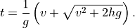
We can write this as a function:

[17]:

from math import sqrt

def drop_time(height, speed, gravity):
    """
    Return how long it takes an object released from a height h,
    in a gravitational field of strength g, with initial vertical speed v,
    to hit the ground.

    Parameters
    ----------

    height : float
        Initial height h
    speed : float
        Initial vertical speed v
    gravity : float
        Gravitional field strength g

    Returns
    -------

    t : float
        Time the object hits the ground
    """

    return (speed + sqrt(speed**2 + 2.0*height*gravity)) / gravity

But when we start using it, it can be a bit confusing:

[18]:

print(drop_time(10.0, 0.0, 9.8))
print(drop_time(10.0, 1.0, 9.8))
print(drop_time(100.0, 9.8, 15.0))

1.4285714285714284
1.5342519232263467
4.362804694292706

Is that last case correct? Did we really want to change the gravitational field, whilst at the same time using an initial velocity of exactly the value we expect for $g$ ?

A far clearer use of the function comes from using keyword arguments. This is where we explicitly use the name of the function arguments. For example:

[19]:

print(drop_time(height=10.0, speed=0.0, gravity=9.8))

1.4285714285714284

The result is exactly the same, but now it’s explicitly clear what we’re doing.

Even more useful: when using keyword arguments, we don’t have to ensure that the order we use matches the order of the function definition:

[20]:

print(drop_time(height=100.0, gravity=9.8, speed=15.0))

6.300406486742956

This is the same as the confusing case above, but now there is no ambiguity. Whilst it is good practice to match the order of the arguments to the function definition, it is only needed when you don’t use the keywords. Using the keywords is always useful.

What if we said that we were going to assume that the gravitational field strength $g$ is nearly always going to be that of Earth, $9.8$ ms ${}^{-2}$ ? We can re-define our function using a default argument:

[21]:

def drop_time(height, speed, gravity=9.8):
    """
    Return how long it takes an object released from a height h,
    in a gravitational field of strength g, with initial vertical speed v,
    to hit the ground.

    Parameters
    ----------

    height : float
        Initial height h
    speed : float
        Initial vertical speed v
    gravity : float
        Gravitional field strength g

    Returns
    -------

    t : float
        Time the object hits the ground
    """

    return (speed + sqrt(speed**2 + 2.0*height*gravity)) / gravity

Note that there is only one difference here, in the very first line: we state that gravity=9.8. What this means is that if this function is called and the value of gravity is not specified, then it takes the value 9.8.

For example:

[22]:

print(drop_time(10.0, 0.0))
print(drop_time(height=50.0, speed=1.0))
print(drop_time(gravity=15.0, height=50.0, speed=1.0))

1.4285714285714284
3.2980530129318018
2.649516083708069

So, we can still give a specific value for gravity when we don’t want to use the value 9.8, but it isn’t needed if we’re happy for it to take the default value of 9.8. This works both if we use keyword arguments and if not, with certain restrictions.

Some things to keep in mind.

Default arguments can only be used without specifying the keyword if they come after arguments without defaults. It is a very strong convention that arguments with a default come at the end of the argument list.
The value of default arguments can be pretty much anything, but care should be taken to get the behaviour you expect. In particular, it is strongly discouraged to allow the default value to be anything that might change, as this can lead to odd behaviour that is hard to find. In particular, allowing a default value to be a container such as a list (seen below) can lead to unexpected behaviour. See, for example, this discussion, pointing out why, and that the value of the default argument is fixed when the function is defined, not when it’s called.

Printing and strings¶

We have already seen the print function used multiple times. It displays its argument(s) to the screen when called, either from the console or from within a program. It prints some representation of what it is given in the form of a string: it converts simple numbers and other objects to strings that can be shown on the screen. For example:

[23]:

import math
x = 1.2
name = "Alice"
print("Hello")
print(6)
print(name)
print(x)
print(math.pi)
print(math.sin(x))
print(math.sin)
print(math)

Hello
6
Alice
1.2
3.141592653589793
0.9320390859672263
<built-in function sin>
<module 'math' from '/Users/ih3/anaconda/envs/labs/lib/python3.5/lib-dynload/math.so'>

We see that variables are converted to their values (such as name and math.pi) and functions are called to get values (such as math.sin(x)), which are then converted to strings displayed on screen. However, functions (math.sin) and modules (math) are also “printed”, in that a string saying what they are, and where they come from, is displayed.

Often we want to display useful information to the screen, which means building a message that is readable and printing that. There are many ways of doing this: here we will just look at the format command. Here is an example:

[24]:

print("Hello {}. We set x={}.".format(name, x))

Hello Alice. We set x=1.2.

The format command takes the string (here "Hello {}. We set x={}.") and replaces the {} with the values of the variables (here name and x in order).

We can use the format command in this way for anything that has a string representation. For example:

[25]:

print ("The function {} applied to x={} gives {}".format(math.sin, x, math.sin(x)))

The function <built-in function sin> applied to x=1.2 gives 0.9320390859672263

There are many more ways to use the format command which can be helpful.

We note that format is a function, but a function applied to the string before the dot. This type of function is called a method, and we shall return to them later.

We have just printed a lot of strings out, but it is useful to briefly talk about what a string is.

In Python a string is not just a sequence of characters. It is a Python object that contains additional information that “lives on it”. If this information is a constant property it is called an attribute. If it is a function it is called a method. We can access this information (using the “dot” notation as above) to tell us things about the string, and to manipulate it.

Here are some basic string methods:

[26]:

name = "Alice"
number = "13"
sentence = "   a  b  c d     e  "
print(name.upper())
print(name.lower())
print(name.isdigit())
print(number.isdigit())
print(sentence.strip())
print(sentence.split())

ALICE
alice
False
True
a  b  c d     e
['a', 'b', 'c', 'd', 'e']

The use of the “dot” notation appears here. We saw this with accessing functions in modules and packages above; now we see it with accessing attributes and methods. It appears repeatedly in Python. The format method used above is particularly important for our purposes, but there are a lot of methods available.

There are other ways of manipulating strings.

We can join two strings using the + operator.

[27]:

print("Hello" + "Alice")

HelloAlice

We can repeat strings using the * operator.

[28]:

print("Hello" * 3)

HelloHelloHello

We can convert numbers to strings using the str function.

[29]:

print(str(3.4))

3.4

We can also access individual characters (starting from 0!), or a range of characters:

[30]:

print("Hello"[0])
print("Hello"[2])
print("Hello"[1:3])

H
l
el

We will come back to this notation when discussing lists and slicing.

Note¶

There are big differences between how Python deals with strings in Python 2.X and Python 3.X. Whilst most of the commands above will produce identical output, string handling is one of the major reasons why Python 2.X doesn’t always work in Python 3.X. The ways strings are handled in Python 3.X is much better than in 2.X.

Putting it together¶

We can now combine the introduction of programs with functions. First, create a file called lab1_function.py containing the code

from math import pi

def degrees_to_radians(theta_d):
    """
    Convert an angle from degrees to radians.

    Parameters
    ----------

    theta_d : float
        The angle in degrees.

    Returns
    -------

    theta_r : float
        The angle in radians.
    """
    theta_r = pi / 180.0 * theta_d
    return theta_r

This is almost exactly the function as defined above.

Next, write a second file lab1_use_function.py containing

from lab1_function import degrees_to_radians

print(degrees_to_radians(15.0))
print(degrees_to_radians(30.0))
print(degrees_to_radians(45.0))
print(degrees_to_radians(60.0))
print(degrees_to_radians(75.0))
print(degrees_to_radians(90.0))

This function uses our own function to convert from degrees to radians. To save typing we have used the from <module> import <function> notation. We could have instead written import lab1_function, but then every function call would need to use lab1_function.degrees_to_radians.

This program, when run, will print to the screen the angles $(n \pi)/ 12$ for $n = 1, 2, \dots, 6$ .

Exercise: basic functions¶

Write a function to calculate the volume of a cuboid with edge lengths $a, b, c$ . Test your code on sample values such as

$a=1, b=1, c=1$ (result should be $1$ );
$a=1, b=2, c=3.5$ (result should be $7.0$ );
$a=0, b=1, c=1$ (result should be $0$ );
$a=2, b=-1, c=1$ (what do you think the result should be?).

Write a function to compute the time (in seconds) taken for an object to fall from a height $H$ (in metres) to the ground, using the formula

$h(t) = \frac{1}{2} g t^2.$

Use the value of the acceleration due to gravity $g$ from scipy.constants.g. Test your code on sample values such as

$H = 1$ m (result should be $\approx 0.452$ s);
$H = 10$ m (result should be $\approx 1.428$ s);
$H = 0$ m (result should be $0$ s);
$H = -1$ m (what do you think the result should be?).

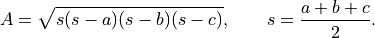
Write a function that computes the area of a triangle with edge lengths $a, b, c$ . You may use the formula

$A = \sqrt{s (s - a) (s - b) (s - c)}, \qquad s = \frac{a + b + c}{2}.$

Construct your own test cases to cover a range of possibilities.

Exercise: Floating point numbers¶

Computers cannot, in principle, represent real numbers perfectly. This can lead to problems of accuracy. For example, if

$x = 1, \qquad y = 1 + 10^{-14} \sqrt{3}$

then it should be true that

$10^{14} (y - x) = \sqrt{3}.$

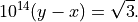
Check how accurately this equation holds in Python and see what this implies about the accuracy of subtracting two numbers that are close together.

Note¶

The standard floating point number holds the first 16 significant digits of a real.

Exercise 2¶

Note: no coding required¶

The standard quadratic formula gives the solutions to

$a x^2 + b x + c = 0$

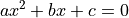
as

$x = \frac{-b \pm \sqrt{b^2 - 4 a c}}{2 a}.$

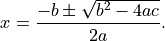
Show that, if 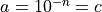$a = 10^{-n} = c$ and $b = 10^n$ then

$x = \frac{10^{2 n}}{2} \left( -1 \pm \sqrt{1 - 4 \times 10^{-4n}} \right).$

Using the expansion (from Taylor’s theorem)

$\sqrt{1 - 4 \times 10^{-4 n}} \simeq 1 - 2 \times 10^{-4 n} + \dots, \qquad n \gg 1,$

show that

$x \simeq -10^{2 n} + 10^{-2 n} \quad \text{and} \quad -10^{-2n}, \qquad n \gg 1.$

Exercise 3¶

Note: no coding required¶

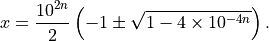
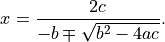
By multiplying and dividing by 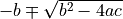$-b \mp \sqrt{b^2 - 4 a c}$ , check that we can also write the solutions to the quadratic equation as

$x = \frac{2 c}{-b \mp \sqrt{b^2 - 4 a c}}.$

Exercise 4¶

Using Python, calculate both solutions to the quadratic equation

$10^{-n} x^2 + 10^n x + 10^{-n} = 0$

for $n = 3$ and $n = 4$ using both formulas. What do you see? How has floating point accuracy caused problems here?

Exercise 5¶

The standard definition of the derivative of a function is

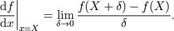
$\left. \frac{\text{d} f}{\text{d} x} \right|_{x=X} = \lim_{\delta \to 0} \frac{f(X + \delta) - f(X)}{\delta}.$

We can approximate this by computing the result for a finite value of $\delta$ :

$g(x, \delta) = \frac{f(x + \delta) - f(x)}{\delta}.$

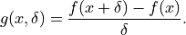
Write a function that takes as inputs a function of one variable, $f(x)$ , a location $X$ , and a step length $\delta$ , and returns the approximation to the derivative given by $g$ .

Exercise 6¶

The function $f_1(x) = e^x$ has derivative with the exact value $1$ at $x=0$ . Compute the approximate derivative using your function above, for $\delta = 10^{-2 n}$ with $n = 1, \dots, 7$ . You should see the results initially improve, then get worse. Why is this?

Programs¶

Using programs and modules¶

Note¶

Functions¶

Printing and strings¶

Note¶

Putting it together¶

Exercise: basic functions¶

Exercise: Floating point numbers¶

Note¶

Exercise 2¶

Note: no coding required¶

Exercise 3¶

Note: no coding required¶

Exercise 4¶

Exercise 5¶

Exercise 6¶

Maths with Python

Navigation

Related Topics