Scientific Python¶

A lot of computational algorithms are expressed using Linear Algebra terminology - vectors and matrices. This is thanks to the wide range of methods within Linear Algebra for solving the sort of problems that computers are good at solving!

Within Python, our first thought may be to represent a vector as a list. But there is a downside: lists do not naturally behave as vectors. For example:

[1]:

x = [1, 2, 3]
y = [4, 9, 16]
print(x+y)

[1, 2, 3, 4, 9, 16]

Similarly, we cannot apply algebraic operations or functions to lists in a straightforward manner that matches our expectations.

However, there is a Python package - numpy - that does give us the behaviour we want.

numpy¶

[2]:

import numpy

numpy is used so frequently that in a lot of cases and online explanations you will see it abbreviated, using import numpy as np. Here we try to avoid that - auto-completion inside spyder means that the additional typing is trivial, and using the full name is clearer.

numpy defines a special type, an array, which can represent vectors, matrices, and other higher-rank objects. Unlike standard Python lists, an array can only contain objects of a single type. The notation to create these objects is straightforward: one easy way is to start with a list:

[3]:

x_numpy = numpy.array(x)
y_numpy = numpy.array(y)
print(x_numpy + y_numpy)
print(x_numpy[0])
print(y_numpy[1:])

[ 5 11 19]
1
[ 9 16]

We see that the array objects behave as we would expect, and accessing elements is exactly the same as for a list. We can also perform other mathematical operations on the whole vector:

[4]:

print(3*x_numpy)
print(numpy.log(x_numpy))
print(x_numpy*y_numpy)
print((x_numpy-1)**2)

[3 6 9]
[ 0.          0.69314718  1.09861229]
[ 4 18 48]
[0 1 4]

Think about these carefully.

The first case is straightforward: all elements of the vector are multiplied by a constant.
The second case applies a function to each element separately. numpy implements a version of most interesting mathematical functions, which are applied directly to each element.
The third case is elementwise multiplication of the vectors. The first component of the answer is the product of the first component of x_numpy with the first component of y_numpy. The second component of the answer is the product of the second component of x_numpy with the second component of y_numpy. We cannot use the * operator to represent matrix multiplication, but must use a function (see below; note that there will be an operator in Python 3.5+, but using it will mean your code is, for now, not widely useable).
The fourth case shows a combination of cases above. The answer is given by elementwise subtraction of 1, then squaring (elementwise) that result.

Defining a matrix can be done by applying the array function to a list of lists:

[5]:

A_numpy = numpy.array([ [1, 2, 3], [4, 5, 6], [7, 8, 0]])
print(A_numpy**2)

[[ 1  4  9]
 [16 25 36]
 [49 64  0]]

We see that for higher rank objects such as matrices, the operations are still performed elementwise.

To multiply a matrix by a vector, or a vector by a vector, in the standard linear algebra sense, we use the numpy.dot function:

[6]:

x_squared = numpy.dot(x_numpy, x_numpy)
A_times_x = numpy.dot(A_numpy, x_numpy)
print(x_squared)
print(A_times_x)

14
[14 32 23]

Note that we have appeared to multiply a matrix by a row vector, and get a row vector back. This is because numpy does not distinguish between row and column vectors, so everything appears as a row vector. (You could define a $n \times 1$ array instead, but there is no advantage).

To actually check the shape and size of numpy arrays, you can directly check their attributes:

[7]:

print(x_numpy.size)
print(x_numpy.shape)
print(A_numpy.size)
print(A_numpy.shape)

3
(3,)
9
(3, 3)

numpy contains a number of very efficient functions for working with arrays, for finding extreme values, and performing linear algebra tasks. Particular functions that are worth knowing, or starting from, are

arange: constructs an array containing increasing integers
linspace: constructs a linearly spaced array
zeros and ones: constructs arrays containing just ones or zeros
diag: extracts the diagonal of a matrix, or build a matrix with just diagonal entries
mgrid: constructs matrices from vectors for 3d plots
random.rand: constructs an array of random numbers.

Linear algebra¶

numpy also defines a number of linear algebra functions. However, a more comprehensive set of functions, which is better maintained and often more efficient, is given by scipy:

[8]:

from scipy import linalg

[9]:

print(linalg.solve(A_numpy, x_numpy))
print(linalg.det(A_numpy))

[-0.33333333  0.66666667  0.        ]
27.0

In addition to solving linear systems and computing determinants, you can also factorize matrices and generally do most linear algebra operations that you need. The scipy documentation is comprehensive, and has a specific section on Linear Algebra, as well as a section in the tutorial. Johansson also has a tutorial on scipy in general.

Working with files¶

Often we will want to work with data - constants, parameters, initial conditions, measurements, and so on. numpy provides ways to work with data stored in files - either reading them in or writing them out. A list of “File I/O routines” is available, but the two key routines are `loadtxt <http://docs.scipy.org/doc/numpy/reference/generated/numpy.loadtxt.html#numpy.loadtxt>`__ and `savetxt <http://docs.scipy.org/doc/numpy/reference/generated/numpy.savetxt.html#numpy.savetxt>`__.

As a simple example we take our matrix A_numpy above and save it to a file:

[10]:

numpy.savetxt('A_numpy.txt', A_numpy)

We can then check the contents of that file (you should open the file on your machine to check):

[11]:

!cat A_numpy.txt

1.000000000000000000e+00 2.000000000000000000e+00 3.000000000000000000e+00
4.000000000000000000e+00 5.000000000000000000e+00 6.000000000000000000e+00
7.000000000000000000e+00 8.000000000000000000e+00 0.000000000000000000e+00

Finally, we can read the contents of that file into a new variable and check that it matches:

[12]:

A_from_file = numpy.loadtxt('A_numpy.txt')
print(A_from_file == A_numpy)

[[ True  True  True]
 [ True  True  True]
 [ True  True  True]]

Plotting¶

There are many Python plotting libraries depending on your purpose. However, the standard general-purpose library is matplotlib. This is often used through its pyplot interface.

This is a quick recap of the basic plotting commands, but using numpy as well.

[13]:

from matplotlib import pyplot

[14]:

%matplotlib inline
from matplotlib import rcParams
rcParams['figure.figsize']=(12,9)

[15]:

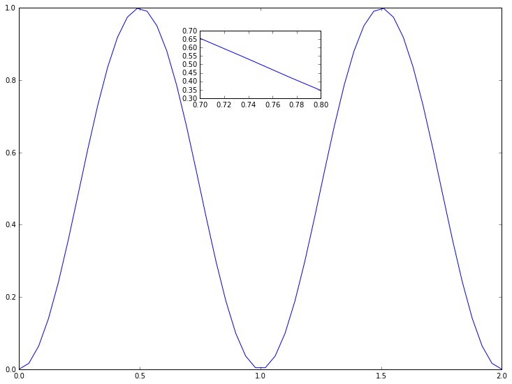
x = numpy.linspace(0, 2.0)
y = numpy.sin(numpy.pi*x)**2
pyplot.plot(x, y)
pyplot.show()

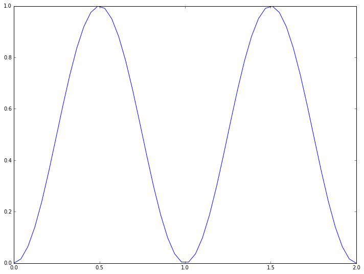
This plotting interface is straightforward, but the results are not particularly nice. The following commands illustrate some of the ways of improving the plot:

[16]:

x = numpy.linspace(0, 2.0)
y = numpy.sin(numpy.pi*x)**2
pyplot.plot(x, y, marker='x', markersize=10, linestyle=':', linewidth=3,
            color='b', label=r'$\sin^2(\pi x)$')
pyplot.legend(loc='lower right')
pyplot.xlabel(r'$x$')
pyplot.ylabel(r'$y$')
pyplot.title('A basic plot')
pyplot.show()

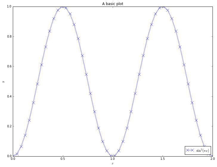
Whilst most of the commands are self-explanatory, a brief note should be made of the strings line r'$x$'. These strings are in LaTeX format, which is the standard typesetting method for professional-level mathematics. The $ symbols surround mathematics. The r before the definition of the string says that the following string will be “raw”: that backslash characters should be left alone. Then, special LaTeX commands have a backslash in front of them: here we use \pi and \sin. We can also use ^ to denote superscripts (used here), _ to denote subscripts, and use {} to group terms.

By combining these basic commands with other plotting types (semilogx and loglog, for example), most simple plots can be produced quickly.

Saving figures¶

If you want to save the figure to a file, instead of printing it to the screen, use the `savefig <http://matplotlib.org/api/pyplot_api.html#matplotlib.pyplot.savefig>`__ command instead of the show command. For example, try:

[17]:

x = numpy.linspace(0, 2.0)
y = numpy.sin(numpy.pi*x)**2
pyplot.plot(x, y, marker='^', markersize=10, linestyle='-.', linewidth=3,
            color='b', label=r'$\sin^2(\pi x)$')
pyplot.legend(loc='lower right')
pyplot.xlabel(r'$x$')
pyplot.ylabel(r'$y$')
pyplot.title('A basic plot')
pyplot.savefig('simple_plot.png')

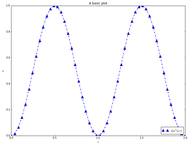
We can then check the file on disk (you should open the file on your machine to check):

[18]:

from IPython.display import Image
Image('simple_plot.png')

[18]:

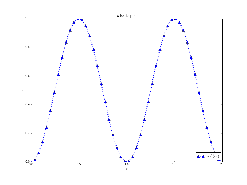
The type of the file is taken from the extension. Here we have used a png file, but svg and pdf output will also work.

Object-based approach¶

To get a more detailed control over the plot it’s better to look at the objects that matplotlib is producing. Remember, when we talked about classes we said that it is an object with attributes and methods (functions) that are accessed using dot notation. Here are steps to completely control the plot.

First we define a figure object. We do not have to define the figure class - it is defined within matplotlib itself, along with a lot of useful methods. We call the constructor of the figure object in the same way as in the previous section, by calling pyplot.figure(). We can and will control its size (the units default to inches) by passing additional arguments to the constructor:

[19]:

fig = pyplot.figure(figsize=(12, 9))

<matplotlib.figure.Figure at 0x10b0e5240>

We will then define two axes on this figure. The numbers refers to the positions of the edges of the axes with respect to the figure window (between 0 and 1):

[20]:

axis1 = fig.add_axes([0.1, 0.1, 0.8, 0.8]) # left, bottom, width, height
axis2 = fig.add_axes([0.4, 0.7, 0.2, 0.15])

We will then add data to the both axes:

[21]:

axis1.plot(x, y)
axis2.plot(x, y)

[21]:

[<matplotlib.lines.Line2D at 0x10b0416a0>]

We will then set the range of the second axis:

[22]:

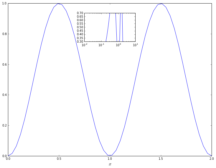
axis2.set_xbound(0.7, 0.8)
axis2.set_ybound(0.3, 0.7)

Finally, we’ll see what it looks like:

[23]:

fig

[23]:

Each axis contains additional objects that can be modified.

[24]:

axis2.set_xscale('log')
axis1.set_xlabel(r'$x$', fontsize=16)
fig

[24]:

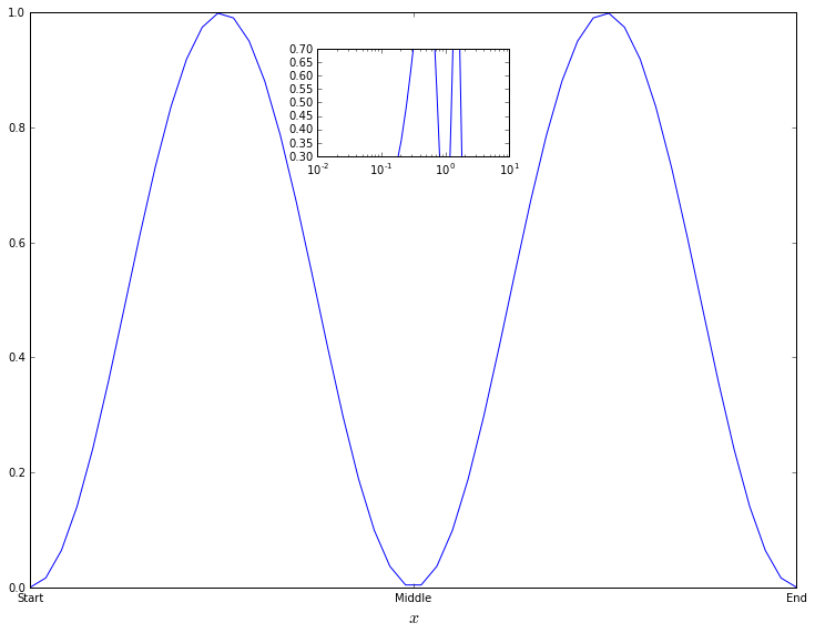
[25]:

axis1.set_xticks([0, 1, 2])
axis1.set_xticklabels(['Start', 'Middle', 'End'])
fig

[25]:

Adding multiple axes by hand is often annoying (although sometimes necessary). There are a number of tools that can be used to simplify this in standard cases: add_subplot is the standard one. When you want a figure containing multiple subplots all the same size, with r rows and c columns, the command is add_subplot(r, c, <subplot_number>). For example:

[26]:

fig = pyplot.figure(figsize=(12, 9))
x = numpy.linspace(0.0, 1.0)
for subplot in range(1, 7):
    axis = fig.add_subplot(2, 3, subplot)
    axis.plot(x, numpy.sin(numpy.pi*x*subplot))
    axis.set_xlabel(r'$x$')
    axis.set_ylabel(r'$y$')
    axis.set_title(r'$\sin({} \pi x)$'.format(subplot))
fig.tight_layout();

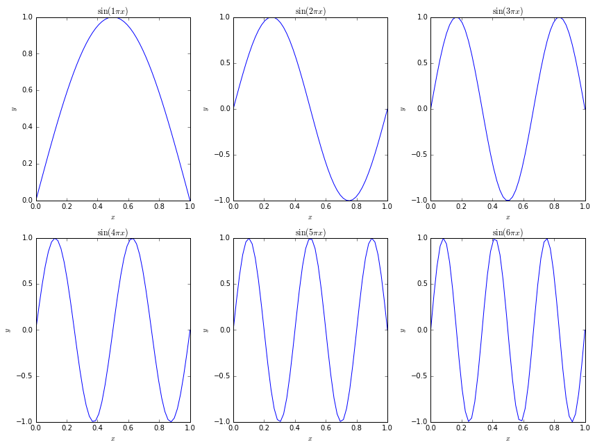
The tight_layout function call at the end ensures that the axis labels and titles do not overlap with other subplots.

Higher dimensions¶

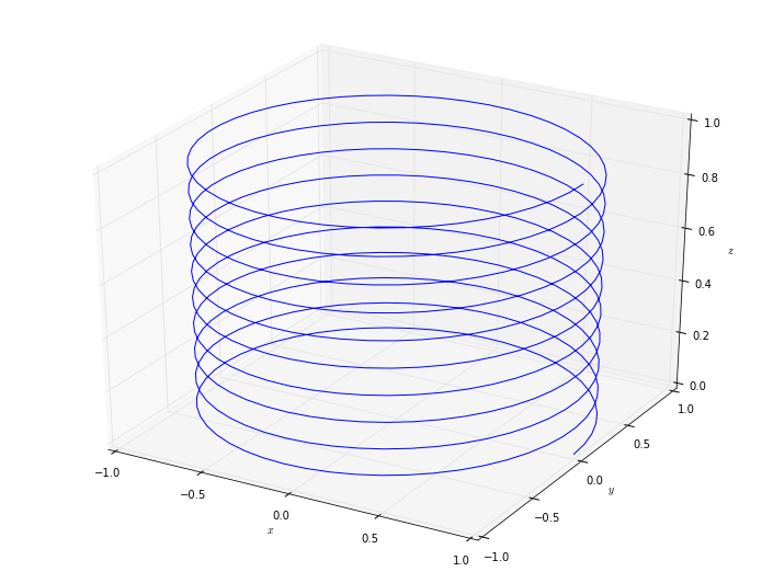
To plot three-dimensional objects, we need to modify the axis so that it knows a third dimension is required. To do this, we import another module and modify the command that sets up the axis object.

[27]:

from mpl_toolkits.mplot3d.axes3d import Axes3D

fig = pyplot.figure(figsize=(12, 9))
axis = fig.add_axes([0.1, 0.1, 0.8, 0.8], projection='3d')

We can then construct, for example, a parametric spiral:

[28]:

t = numpy.linspace(0.0, 10.0, 500)
x = numpy.cos(2.0*numpy.pi*t)
y = numpy.sin(2.0*numpy.pi*t)
z = 0.1*t

axis.plot(x, y, z)
axis.set_xlabel(r'$x$')
axis.set_ylabel(r'$y$')
axis.set_zlabel(r'$z$')
fig

[28]:

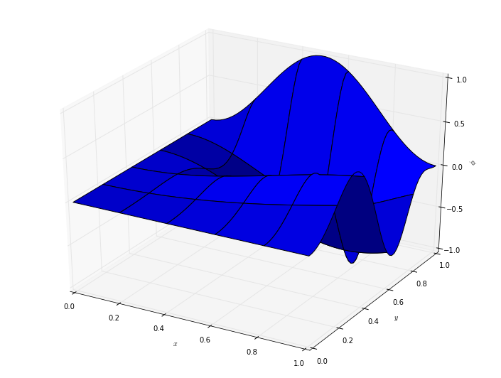
If we want to plot a surface, then we need to construct 2d arrays containing the locations of the $x$ and $y$ coordinates, and a 2d array containing the “height” of the surface. For structured data (ie, where the $x$ and $y$ coordinates lie on a regular grid) the meshgrid function helps. For example, the function

$\phi(x, y) = \sin^2 ( \pi x y ) \cos( 2 \pi y^2 ), \qquad x \in [0, 1], \quad y \in [0, 1],$

would be plotted using

[29]:

fig = pyplot.figure(figsize=(12, 9))
axis = fig.add_axes([0.1, 0.1, 0.8, 0.8], projection='3d')

x = numpy.linspace(0.0, 1.0)
y = numpy.linspace(0.0, 1.0)

X, Y = numpy.meshgrid(x, y)
# x, y are vectors
# X, Y are 2d arrays

phi = numpy.sin(numpy.pi*X*Y)**2 * numpy.cos(2.0*numpy.pi*Y**2)

axis.plot_surface(X, Y, phi)
axis.set_xlabel(r'$x$')
axis.set_ylabel(r'$y$')
axis.set_zlabel(r'$\phi$');

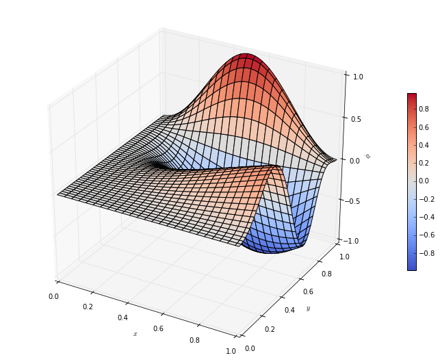
There are a lot of options to modify the appearance of this plot. Important ones include the colormap (note the US spelling), which requires importing the cm module from matplotlib, and the stride parameters changing the appearance of the grid. For example

[30]:

from matplotlib import cm

fig = pyplot.figure(figsize=(12, 9))
axis = fig.add_axes([0.1, 0.1, 0.8, 0.8], projection='3d')

p = axis.plot_surface(X, Y, phi, rstride=1, cstride=2, cmap = cm.coolwarm)
axis.set_xlabel(r'$x$')
axis.set_ylabel(r'$y$')
axis.set_zlabel(r'$\phi$')
fig.colorbar(p, shrink=0.5);

scipy¶

scipy is a package for scientific Python, and contains many functions that are essential for mathematics. It works particularly well with numpy. We briefly introduced it above for tackling Linear Algebra problems, but it also includes

Scientific constants
Integration and ODE solvers
Interpolation
Optimization and root finding
Statistical functions

and much more.

Integration¶

The numerical quadrature problem involves solving the definite integral

$\int_a^b f(x) \, \text{d} x,$

or a suitable generalization. scipy has a module, scipy.integrate, that includes a number of functions to solve these types of problems. For example, to solve

$I = \int_0^{\pi} \sin^2(x) \, \text{d} x,$

the quad function can be used as:

[31]:

from numpy import sin
from scipy.integrate import quad

def integrand(x):
    """
    The integrand \sin^2(x).

    Parameters
    ----------

    x : real (list)
        The point(s) at which the integrand is evaluated

    Returns
    -------

    integrand : real (list)
        The integrand evaluated at x
    """

    return sin(x)**2

result = quad(integrand, 0.0, numpy.pi)
print("The result is {}.".format(result))

The result is (1.5707963267948966, 1.743934249004316e-14).

The steps we have taken are:

Define the integrand by defining a function. This function takes the points at which the integrand is evaluated. By using numpy we can do this with a single command.
Import the quad function.
Call the quad function, passing the function defining the integrand, and the lower and upper limits.

The result we get back, as seen from the screen output, is not just $I$ . It is a tuple containing both $I$ , and also the accuracy with which quad believes it has computed the result. The quadrature is a numerical approximation, so can never be perfect. You should check this error estimate to ensure the result is “good enough” for your purposes.

We can also pass additional parameters if needed. Consider the problem

$I_a = \int_0^{\pi} \sin^2 (a x) \, \text{d} x.$

If we wanted to solve this for many values of $a$ , say $a = 1, 2, \dots, 5$ , we could create a function taking a parameter, and then pass that parameter through:

[32]:

from numpy import sin
from scipy.integrate import quad

def integrand_param(x, a):
    """
    The integrand \sin^2(a x).

    Parameters
    ----------

    x : real (list)
        The point(s) at which the integrand is evaluated
    a : real
        The parameter for the integrand

    Returns
    -------

    integrand : real (list)
        The integrand evaluated at x
    """

    return sin(a*x)**2

for a in range(1, 6):
    result, accuracy = quad(integrand_param, 0.0, numpy.pi, args=(a,))
    print("For a={}, the result is {}.".format(a, result))

For a=1, the result is 1.5707963267948966.
For a=2, the result is 1.5707963267948966.
For a=3, the result is 1.5707963267948966.
For a=4, the result is 1.5707963267948966.
For a=5, the result is 1.5707963267948968.

Note that when passing the parameters using the args keyword argument, we put the parameters in a tuple. This shows how to pass more than one parameter: keep adding parameters to the argument list, and add them to the tuple. For example, to solve

$I_{a,b} = \int_0^{\pi} \sin^2(ax + b) \, \text{d} x$

we write

[33]:

from numpy import sin
from scipy.integrate import quad

def integrand_param2(x, a, b):
    """
    The integrand \sin^2(a x + b).

    Parameters
    ----------

    x : real (list)
        The point(s) at which the integrand is evaluated
    a : real
        The parameter for the integrand
    b : real
        The second parameter for the integrand

    Returns
    -------

    integrand : real (list)
        The integrand evaluated at x
    """

    return sin(a*x+b)**2

for a in range(1, 3):
    for b in range(3):
        result, accuracy = quad(integrand_param2, 0.0, numpy.pi, args=(a, b))
        print("For a={}, b={}, the result is {}.".format(a, b, result))

For a=1, b=0, the result is 1.5707963267948966.
For a=1, b=1, the result is 1.570796326794897.
For a=1, b=2, the result is 1.570796326794897.
For a=2, b=0, the result is 1.5707963267948966.
For a=2, b=1, the result is 1.5707963267948961.
For a=2, b=2, the result is 1.5707963267948961.

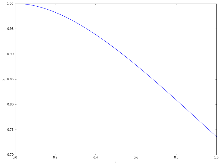
Solving ODEs¶

There is a link between the solution of integrals and the solution of differential equations. Unfortunately, the numerical solution of an ODE is more complex than the solution of an integral. Fortunately, scipy contains a number of methods for these as well.

The methods in scipy solve ODEs of the form

$\frac{\text{d} \vec{y}}{\text{d} t} = \vec{f} \left( \vec{y}, t \right), \qquad \vec{y}(0) = \vec{y}_0.$

For example, the ODE

$\frac{\text{d} y}{\text{d} t} = e^{-t} - y, \qquad y(0) = 1$

has $f(y, t) = e^{-t} - y$ .

The method for using scipy is similar to the integration case.

Define a function that specifies the system, by defining the RHS.
Import the function that solves ODEs (odeint)
Call the function, passing the RHS function, the initial data $\vec{y}_0$ , the times at which the solution is needed, and any parameters.

To solve our example, we use:

[34]:

from numpy import exp
from scipy.integrate import odeint

def dydt(y, t):
    """
    Defining the ODE dy/dt = e^{-t} - y.

    Parameters
    ----------

    y : real
        The value of y at time t (the current numerical approximation)
    t : real
        The current time t

    Returns
    -------

    dydt : real
        The RHS function defining the ODE.
    """

    return exp(-t) - y

t = numpy.linspace(0.0, 1.0)
y0 = [1.0]

y = odeint(dydt, y0, t)
print("The shape of the result is {}.".format(y.shape))
print("The value of y at t=1 is {}.".format(y[-1,0]))

The shape of the result is (50, 1).
The value of y at t=1 is 0.7357588629292717.

Note that the result for $y$ is not a vector, but a two dimensional array. This is because scipy will solve a general system of ODEs. This scalar case is a system of size $1$ , but it still returns an array. To solve a system, the RHS function must take a vector for y, return a vector for dydt, and the initial data y0 must be a vector. All these vectors must be the same size.

The output is the numerical approximation to $y$ at the input times $t$ , and can be immediately plotted:

[35]:

pyplot.plot(t, y[:,0])
pyplot.xlabel(r'$t$')
pyplot.ylabel(r'$y$')
pyplot.show()

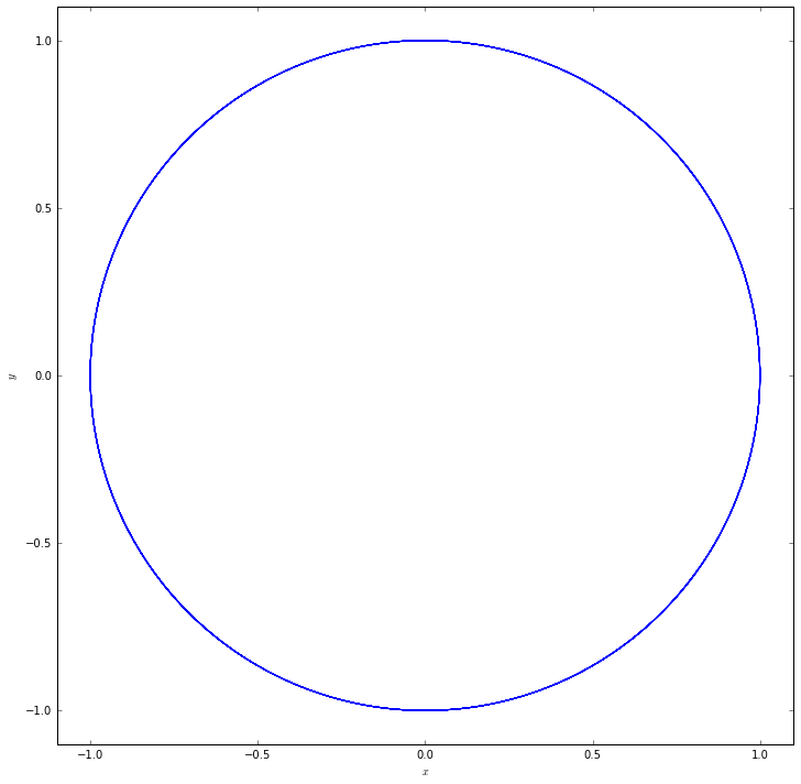
Passing parameters is also similar to the integration case. For example, consider the problem

$\frac{\text{d}}{\text{d} t} \begin{pmatrix} x \\ y \end{pmatrix} = \begin{pmatrix} -y + \alpha \\ x \end{pmatrix}, \qquad \begin{pmatrix} x \\ y \end{pmatrix}(0) = \begin{pmatrix} 1 \\ 0 \end{pmatrix}.$

If $\alpha$ is zero, the solution is a circle in the $x, y$ plane. We solve this using odeint, denoting the state vector $\vec{z} = (x, y)^T$ :

[36]:

import numpy
from scipy.integrate import odeint

def dzdt(z, t, alpha):
    """
    Defining the ODE dz/dt.

    Parameters
    ----------

    z : real, list
        The value of z at time t (the current numerical approximation)
    t : real
        The current time t
    alpha : real
        Parameter

    Returns
    -------

    dzdt : real
        The RHS function defining the ODE.
    """

    dzdt = numpy.zeros_like(z)
    x, y = z
    dzdt[0] = -y + alpha
    dzdt[1] = x

    return dzdt

t = numpy.linspace(0.0, 50.0, 1000)
z0 = [1.0, 0.0]
alpha = 1e-5

z = odeint(dzdt, z0, t, args=(alpha,))

[37]:

fig = pyplot.figure(figsize=(12,12))
ax = fig.add_subplot(1,1,1)
ax.plot(z[:,0], z[:,1])
ax.set_xlabel(r'$x$')
ax.set_ylabel(r'$y$')
ax.set_xlim(-1.1, 1.1)
ax.set_ylim(-1.1, 1.1);

Exercise: Lorenz attractor¶

The Lorenz system is a set of ordinary differential equations which can be written

$\frac{\text{d} \vec{v}}{\text{d} \vec{t}} = \vec{f}(\vec{v})$

where the variables in the state vector $\vec{v}$ are

$\vec{v} = \begin{pmatrix} x(t) \\ y(t) \\ z(t) \end{pmatrix}$

and the function defining the ODE is

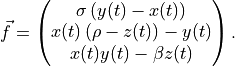
$\vec{f} = \begin{pmatrix} \sigma \left( y(t) - x(t) \right) \\ x(t) \left( \rho - z(t) \right) - y(t) \\ x(t) y(t) - \beta z(t) \end{pmatrix}.$

The parameters $\sigma, \rho, \beta$ are all real numbers.

Exercise 1¶

Write a function dvdt(v, t, params) that returns $\vec{f}$ given $\vec{v}, t$ and the parameters $\sigma, \rho, \beta$ .

Exercise 2¶

Fix $\sigma=10, \beta=8/3$ . Set initial data to be $\vec{v}(0) = \vec{1}$ . Using scipy, specifically the odeint function of scipy.integrate, solve the Lorenz system up to $t=100$ for $\rho=13, 14, 15$ and $28$ .

Plot your results in 3d, plotting $x, y, z$ .

Exercise 3¶

Fix $\rho = 28$ . Solve the Lorenz system twice, up to $t=40$ , using the two different initial conditions $\vec{v}(0) = \vec{1}$ and $\vec{v}(0) = \vec{1} + \vec{10^{-5}}$ .

Show four plots. Each plot should show the two solutions on the same axes, plotting $x, y$ and $z$ . Each plot should show $10$ units of time, ie the first shows $t \in [0, 10]$ , the second shows $t \in [10, 20]$ , and so on.

This shows the sensitive dependence on initial conditions that is characteristic of chaotic behaviour.

Exercise: Mandelbrot¶

The Mandelbrot set is also generated from a sequence, $\{ z_n \}$ , using the relation

$z_{n+1} = z_n^2 + c, \qquad z_0 = 0.$

The members of the sequence, and the constant $c$ , are all complex. The point in the complex plane at $c$ is in the Mandelbrot set only if the $|z_n| < 2$ for all members of the sequence. In reality, checking the first 100 iterations is sufficient.

Note: the Python notation for a complex number $x + \text{i} y$ is x + yj: that is, j is used to indicate $\sqrt{-1}$ . If you know the values of x and y then x + yj constructs a complex number; if they are stored in variables you can use complex(x, y).

Exercise 1¶

Write a function that checks if the point $c$ is in the Mandelbrot set.

Exercise 2¶

Check the points $c=0$ and $c=\pm 2 \pm 2 \text{i}$ and ensure they do what you expect. (What should you expect?)

Exercise 3¶

Write a function that, given $N$

generates an $N \times N$ grid spanning $c = x + \text{i} y$ , for $-2 \le x \le 2$ and $-2 \le y \le 2$ ;
returns an $N\times N$ array containing one if the associated grid point is in the Mandelbrot set, and zero otherwise.

Exercise 4¶

Using the function imshow from matplotlib, plot the resulting array for a $100 \times 100$ array to make sure you see the expected shape.

Exercise 5¶

Modify your functions so that, instead of returning whether a point is inside the set or not, it returns the logarithm of the number of iterations it takes. Plot the result using imshow again.

Exercise 6¶

Try some higher resolution plots, and try plotting only a section to see the structure. Note this is not a good way to get high accuracy close up images!

Exercise: The shortest published Mathematical paper¶

A candidate for the shortest mathematical paper ever shows the following result:

$27^5 + 84^5 + 110^5 + 133^5 = 144^5.$

This is interesting as

This is a counterexample to a conjecture by Euler … that at least $n$ $n$ th powers are required to sum to an $n$ th power, $n > 2$ .

Exercise 1¶

Using Python, check the equation above is true.

Exercise 2¶

The more interesting statement in the paper is that

$27^5 + 84^5 + 110^5 + 133^5 = 144^5.$

is

the smallest instance in which four fifth powers sum to a fifth power.

Interpreting “the smallest instance” to mean the solution where the right hand side term (the largest integer) is the smallest, we want to use Python to check this statement.

We are going to need to generate all possible combinations of four integers $a, b, c, d$ and test if $a^5 + b^5 + c^5 + d^5$ matches $e^5$ where $e$ is another integer.

The problem is the number of combinations grows very fast - the standard formula says that for a list of length $\ell$ there are

$\begin{pmatrix} \ell \\ k \end{pmatrix} = \frac{\ell!}{k! (\ell-k)!}$

combinations of length $k$ . For $k=4$ as needed here we will have $\ell (\ell-1) (\ell-2) (\ell-3) / 24$ combinations.

Show, by getting Python to compute the number of combinations $N = \begin{pmatrix} \ell \\ 4 \end{pmatrix}$ that $N$ grows roughly as $\ell^4$ . To do this, plot the number of combinations and $\ell^4$ on a log-log scale. Restrict to $\ell \le 50$ .

You may find the combinations function from the itertools package useful.

Exercise 3¶

With 17 million combinations to work with, we’ll need to be a little careful how we compute. To check the interesting statement in the paper,

Construct a numpy array containing all integers in $1, \dots, 144$ to the fifth power.
Construct a list of all combinations of four elements from this array.
Construct a list of sums of all these combinations.
Loop over one list and check if the entry appears in the other list (ie, use the in keyword).

By printing out any entries that pass this check, you should see only the solution given in the paper.

Scientific Python¶

numpy¶

Linear algebra¶

Working with files¶

Plotting¶

Saving figures¶

Object-based approach¶

Higher dimensions¶

Further reading¶

scipy¶

Integration¶

Solving ODEs¶

Further reading¶

Exercise: Lorenz attractor¶

Exercise 1¶

Exercise 2¶

Exercise 3¶

Exercise: Mandelbrot¶

Exercise 1¶

Exercise 2¶

Exercise 3¶

Exercise 4¶

Exercise 5¶

Exercise 6¶

Exercise: The shortest published Mathematical paper¶

Exercise 1¶

Exercise 2¶

Exercise 3¶

Maths with Python

Navigation

Related Topics